Welcome to SAXS_routines’s documentation!
SAXS analysis routines
The package contains Python-based analysis routines for small-angle X-ray scattering data.
The routines are initially intended to be used with SAXS data, where a liquid chromatography column was connected before the injection into the capillary, but can be used with standard measurement data as well.
Installation:
Simply use python3 setup.py install.
Quick start
The experimental data can be imported using the functions present in the data_parsers module. For instance, a size-exclusion chromatography and small-angle scattering (SEC-SANS) experiment file performed on the BM29 beamline at the ESRF can be imported using:
from saxs_routines.data_parsers.esrf_bm29 import read_HPLC

data = read_HPLC('my_data_file.h5', name='my_protein_name')
The function returns an instance of the sample.Sample class
which is a subclass of the NumPy ndarray. Hence, various operations are
available with the data (slicing, mean, addition, division, transpose, …).
Along with the intensities, the class sample.Sample stores various
metadata such as errors, incoming beam intensity, beamline name, momentum
transfer q-values or time (see documentation for details).
An important feature of the class sample.Sample is that the error
propagation is done automatically for most of the operators applied on the
data.
Also, the momentum transfer q-values and the elution time are automatically
sliced with the data.
from saxs_routines.data_analysis import FindPeaks

peaks = FindPeaks(data)
peaks.run()

sample = peaks.get_sub_arrays()[0]  # select the first peak found

# select the buffer region (first 50 minutes) and perform the subtraction
buffer = data.get_time_range(0, 50)
sample = sample - 0.95 * buffer
The treated data can be saved in text format using the following:
The class sample.Sample also contains a method for quick plotting:
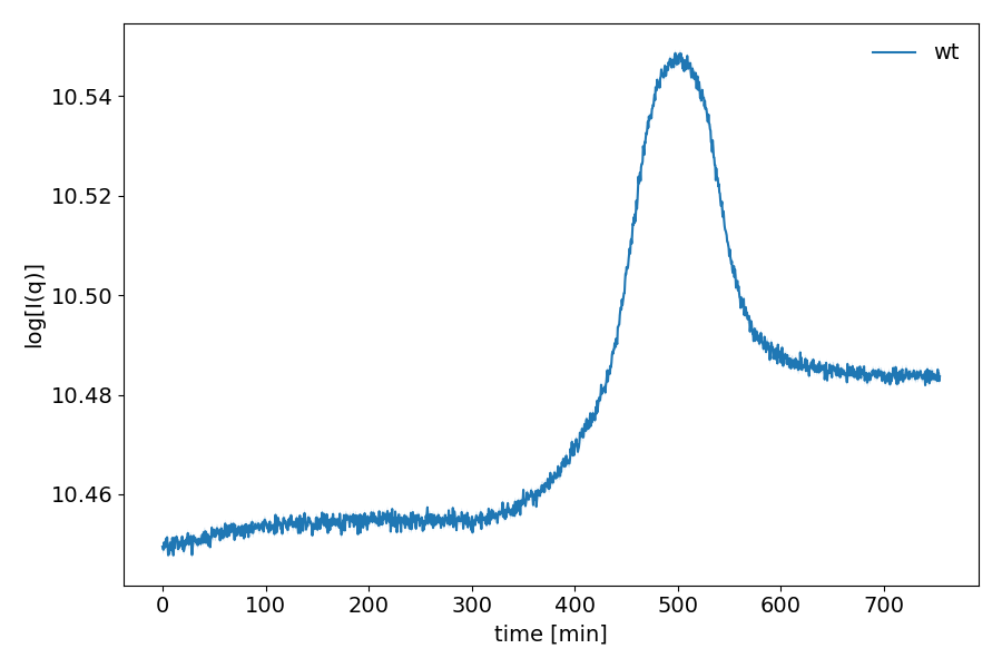
# for a log plot of the signal integrated over q
data.sum(1).plot('log')
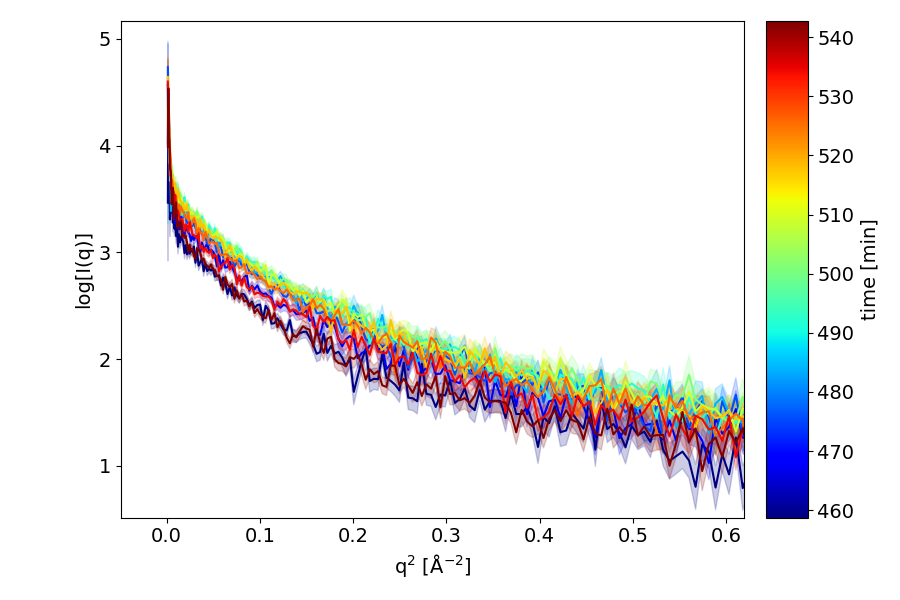
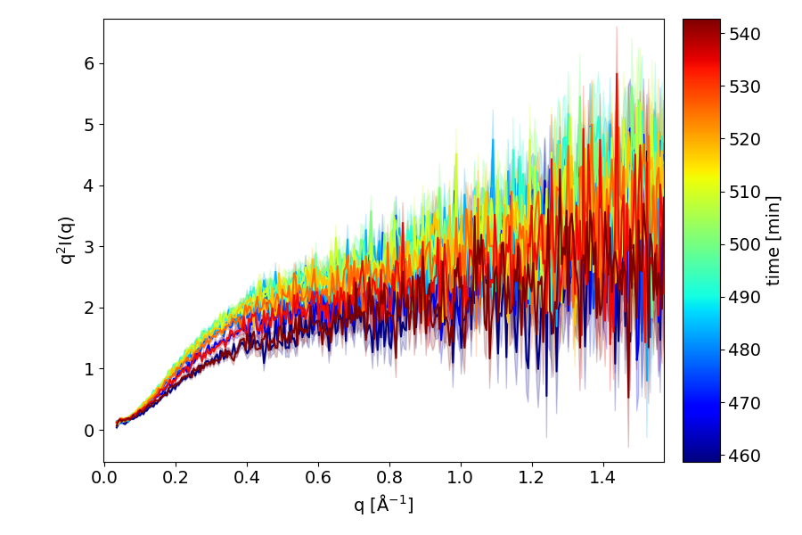
# for a guinier and a kratky plot of the signal over time
data.plot('guinier', axis=1, max_lines=10, new_fig=True)
data.plot('kratky', axis=1, max_lines=10, new_fig=True)
To automatically find a peak in a SEC-SANS experiment and subsequently subtract a rescaled buffer signal, you can use:
sample.write_csv('output_file_name')
Additional data analysis routines will be found in data_analysis module.
User-defined model can also be constructed and fitted to the data. To this end, please refer to the documentation of the model module.
Support
In case of bugs or obvious change to be done in the code use GitHub Issues.
Contributions
See contributing.